Bessel functions

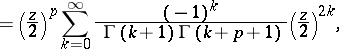
Cylinder functions of the first kind. A Bessel function of order can be defined as the series

(*)

which converges throughout the plane. A Bessel function of order is the solution of the corresponding Bessel equation. If the argument and the order are real numbers, the Bessel function is real, and its graph has the form of a damped vibration (Fig.); if the order is even, the Bessel function is even, if odd, it is odd.

Figure: b015840a
Graphs of the functions and .
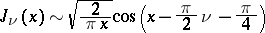
The behaviour of a Bessel function in a neighbourhood of zero is given by the first term of the series (*); for large , the asymptotic representation
holds. The zeros of a Bessel function (i.e. the roots of the equation ) are simple, and the zeros of are situated between the zeros of . Bessel functions of "half-integral" order are expressible by trigonometric functions; in particular
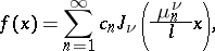
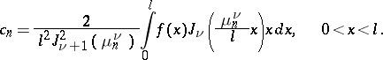
The Bessel functions (where are the positive zeros of , ) form an orthogonal system with weight in the interval . Under certain conditions the following expansion is valid:
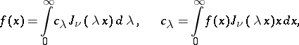
In an infinite interval this expansion is replaced by the Fourier–Bessel integral
The following formulas play an important role in the theory of Bessel functions and their applications:
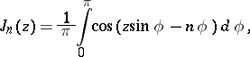
1) the integral representation
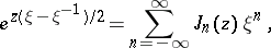
2) the generating function
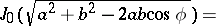
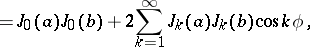
3) the addition theorem for Bessel functions of order zero
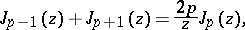
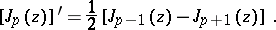
4) the recurrence formulas
For references, see Cylinder functions.

 

Orthogonal Trajectories

We have seen before (see separable equations for example) that the solutions of a differential equation may be given by an implicit equation with a parameter something like

This is an equation describing a family of curves. Whenever we fix the parameter C we get one curve and vice-versa. For example, consider the families of curves

where m and C are parameters. Clearly, we may change the names of the variables and still have the same geometric curves. For example, the above families define the same geometric object as

Note that the first family describes all the lines passing by the origin (0,0) while the second the family describes all the circles centered at the origin (including the limit case when the radius 0 which reduces to the single point (0,0)) (see the pictures below).

and
In this page, we will only use the variables x and y. Any family of curves will be written as

One may ask whether any family of curves may be generated from a differential equation? In general, the answer is no. Let us see how to proceed if the answer were to be yes. First differentiate with respect to x, and get a new equation involving in general x, y, , and C. Using the original equation, we may able to eliminate the parameter C from the new equation.

Example. Find the differential equation satisfied by the family

Answer. We differentiate with respect to x, to get

Since we have

then we get

You may want to do some algebra to make the new equation easy to read. The next step is to rewrite this equation in the explicit form

this is the desired differential equation.

Example. Find the differential equation (in the explicit form) satisfied by the family

Answer. We have already found the differential equation in the implicit form

Algebraic manipulations give

Let us reconsider the example of the two families

If we draw the two families together on the same graph we get

As we see here something amazing happened. Indeed, it is clear that whenever one line intersects one circle, the tangent line to the circle (at the point of intersection) and the line are perpendicular or orthogonal. We say the two curves are orthogonal at the point of intersection.

Definition. Consider two families of curves and . We say that and are orthogonal whenever any curve from intersects any curve from , the two curves are orthogonal at the point of intersection.

For example, we have seen that the families y = m x and are orthogonal. One may then ask the following natural question:

Given a family of curves , is it possible to find a family of curves which is orthogonal to ?
The answer to this question has many implications in many areas such as physics, fluid-dynamics, etc... In general this question is very difficult. But in some cases, we may be able to carry on the calculations and find the orthogonal family. Let us show how.

Consider the family of curves . We assume that an associated differential equation may be found, say

We know that for any curve from the family passing by the point (x,y), the slope of the tangent at this point is f(x,y). Hence the slope of the line perpendicular (or orthogonal) to this tangent is which happens to be the slope of the tangent line to the orthogonal curve passing by the point (x,y). In other words, the family of orthogonal curves are solutions to the differential equation

From this we see what we have to do. Indeed consider a family of curves . In order to find the orthogonal family, we use the following practical steps

Step 1. Find the associated differential equation.

Step 2. Rewrite this differential equation in the explicit form

Step 3. Write down the differential equation associated to the orthogonal family

Step 4. Solve the new equation. The solutions are exactly the family of orthogonal curves.

Step 5. You may be asked to give a geometric view of the two families. Also you may be asked to find a specific curve from the orthogonal family (something like an IVP).

Example. Find the orthogonal family to the family of circles

Answer. First, we look for the differential equation satisfied by the circles. We differentiate with respect to the variable x to get

We rewrite this equation in the explicit form

Next we write down the equation for the orthogonal family

This is a linear as well as a separable equation. If we use the technique of linear equations, we get the integrating factor

which gives

We recognize the family of lines and we confirm our earlier observation (that the two families are indeed orthogonal).

This example is somehow easy and was given here to illustrate the technique.

Example. Find the orthogonal family to the family of circles

Answer. We have seen before that the explicit differential equation associated to the family of circles is

Hence the differential equation for the orthogonal family is

We recognize an homogeneous equation. Let us use the technique developed to solve this kind of equations. Consider the new variable (or equivalently y = x z). Then we have

and

Hence we have

Algebraic manipulations imply

This is a separable equation. The constant solutions are given by

which gives z=0. The non-constant solutions are found once we separate the variables

and then we integrate

Before we perform the integration for the left-hand side, we need to use partial decomposition technique. We have

We will leave the details to you to show that A = 1, B=-2, and C=0. Hence we have

Hence

which is equivalent to

where . Putting all the solutions together we get

Going back to the variable y, we get

which is equivalent to

We recognize a family of circles centered on the y-axis and the line y=0 (the x-axis which was easy to guess, isn't it?)

If we put both families together, we appreciate better the orthogonality of the curves (see the picture below).


[Differential Equations] [First Order D.E.] [Geometry] [Algebra] [Trigonometry ] [Calculus] [Complex Variables] [Matrix Algebra] S.O.S MATHematics home page Mohamed Amine Khamsi